Now that we have learned how to train a neural network (a model) and how to retrieve/create training data, let us review the theory behind optimizing the training of our model.
Training a model is an iterative process: at each iteration, the model estimates the output, computes the error in its estimate (loss), collects the derivatives of the error with respect to its parameters, and optimizes these parameters using gradient descent.
Gradient descent (reminder)
Gradient descent is an algorithm used to find the minimum of a function.
Intuitive approach:
- Intuitively, you can imagine being a skier on a mountain. You are trying to find the lowest point in altitude (i.e., a minimum altitude).
- The approach to find this minimum is to face downhill and simply move forward for 5 minutes.
- So, 5 minutes later, you are at another point and you repeat the previous step.
- And so on until you reach the lowest point.

Mathematical approach:
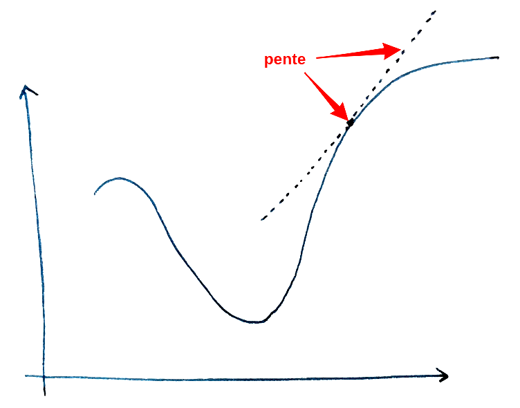
- The slope of the mountain corresponds to the derivative. And the derivative value corresponds to the steepness of the slope at a given point.
- Therefore, a large derivative indicates a steep slope. Likewise, if the derivative is small, then the slope is gentle. Finally, a zero derivative corresponds to flat ground.
- As for the sign of the derivative, you move in the opposite direction of the slope. More concretely, a positive derivative indicates a slope that goes down to the left, and a negative derivative indicates a slope that goes down to the right.
- Once the direction has been determined (left or right), it remains to determine the step size (do we move for 5 minutes, 10 minutes, …?). Ideally, the step should be as small as possible to determine whether we have found the minimum as reliably as possible. The issue with this approach is the computational cost: the computation will be very slow. Conversely, a step that is too large will cause us to miss the minimum. We therefore need to find a balance, which is done by specifying a learning rate (learning_rate), which we will cover later.
Combined approaches:
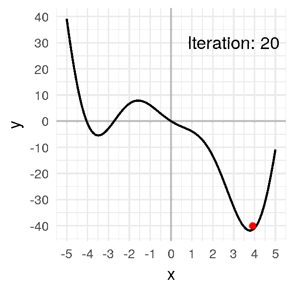
- We can represent the mountain described in the intuitive approach with the following function: f(x) = 2x²cos(x) – 5x. We will limit our study to the interval [-5,5].
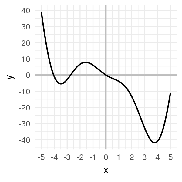
- Visually, the minimum is located around x ≈ 3.8, for a minimum value of approximately y ≈ -42.
- We will therefore apply gradient descent to find this minimum.
To do so, we start by taking an initial x (x0) at random. x0 = -1 -> f(x0) = 6.08)
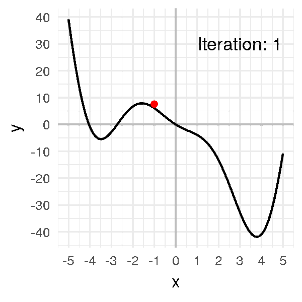
We then compute the slope value at this point (the derivative f'(x0)). f'(-1) = -2sin(-1)-4cos(-1)-5 ≈ -5.47827
We “move” in the direction opposite to the slope: x1 = x0 − αf'(x0) (with α = learning_rate = 0.05). x1 ≈ -0.72609
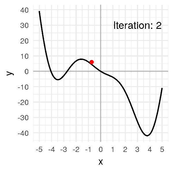
We then repeat the operation until we find xmin. xmin = 3.8
Hyperparameters
This optimization process can be directly influenced by the developer through hyperparameters. These hyperparameters are adjustable parameters that impact model training and its convergence rate. The convergence rate corresponds to how many iterations the model needs to obtain an optimal result.
To train the model, we have 3 hyperparameters:
- Number of epochs epochs_number: the number of times the entire dataset is processed
- Training batch size batch_size: the number of data samples propagated through the network before updating the parameters
- Learning rate learning_rate: how much the model parameters should be updated at each batch/epoch. Smaller values result in a slow learning speed, while larger values can lead to unpredictable behavior during learning. (see “Gradient descent”)
Explanation of hyperparameters
More concretely, we initially have 2 things:
- the model
- a dataset
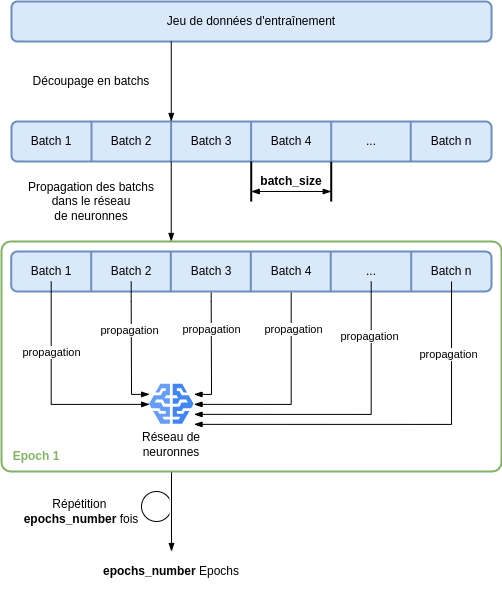
We start by splitting the dataset into subsets, all of the same size. These subsets are called batches, each of size batch_size.
Next, each batch is propagated through the network (passed as input to it). When all batches have been passed through the model, we have completed 1 epoch. The process is then repeated epochs_number times.
These steps can be visualized in the following image.
Model training loop
First of all, the hyperparameters must be defined. For example:
- learning_rate = 1e-3
- batch_size = 64
- epochs = 5
Once the hyperparameters have been defined, the model training and optimization loop can begin. As a reminder, each iteration of this loop is therefore an epoch.
More precisely, each epoch consists of 2 phases:
- training: iterating over the training dataset in order to try to converge towards optimal parameters.
- validation: iterating over the validation dataset to verify that the model performs better and improves.
In the first loop, since our network has not yet been trained, it is very unlikely to produce a good answer/result. We then need to measure the distance between the obtained result and the expected result. This distance is computed using the loss function (loss_function).
The goal is therefore, as the loop iterations progress, to minimize this loss_function in order to obtain a result as close as possible to the expected result. We note here the usefulness of gradient descent which, as explained earlier, is an algorithm used to find the minimum of a function—here, the loss_function.
Optimization therefore consists in updating the parameters at each loop to minimize this loss function. This optimization is encapsulated in an optimizer object that is applied to the model. The latter therefore takes the model hyperparameters as input. In the training loop, optimization is more specifically carried out in 3 steps:
- Call to optimizer.zero_grad(): resetting the model parameter gradients. By default, gradients accumulate; to avoid double counting, we explicitly set them to zero at each iteration.
- Call to loss.backward(): backpropagation of the loss prediction (loss).
- Call to optimizer.step(): adjusting the parameters using the gradients collected during backpropagation.
Conclusion
We have reviewed how to train a data model by introducing the concepts of hyperparameters and highlighting the importance of a good optimizer.
Next time, we will offer you a practical session to code our optimizer and study some of the optimizers provided in PyTorch.
Authors: Mathilde Pommier and Sébastien Da Rocha