Furthermore, these neural networks are also used to classify data or perform forecasts. They are widely utilized in the fields of natural language processing and computer vision, particularly in robotics. Neural networks are therefore present all around us.
However, you may not know what lies behind these networks, which can seem very obscure and complex. If you wish to understand and use these detection, classification, and prediction systems, you must first grasp the concept of neural networks. To do this, we will develop a concrete example.
Concrete Example – Image Classification
A neural network can, for example, be used to classify an image into a specific category. A concrete example would be the application of this technology to the detection and classification of land cover on satellite imagery.
The idea is to provide an image as input to the neural network, which then classifies this image into categories such as “urban” or “rural.” The problem essentially boils down to the following question: “Does my image represent an urban area?”
If we create the network and immediately provide our input image, we will get a random, nonsensical, and highly inaccurate result. We must therefore train our network with a dataset to teach it how to classify images correctly. We provide it with many images of urban and rural areas to teach it to differentiate between them properly.
Different learning methods exist, but the most widespread (and easiest to understand) is supervised learning. This consists of providing the expected result along with the input data. More specifically, each image is annotated with the category “urban” or “rural” so that the network can confirm its results and thus learn from its mistakes. This learning method will be explained in the following sections.
A neural network is based on the functioning of the human brain. It is therefore composed of several neurons interconnected in the following way:
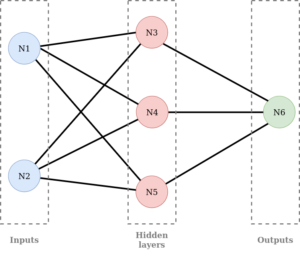
As can be seen, neurons are divided into three families:
– inputs: inputs
– hidden layer neurons: hidden layers
– outputs: outputs
In our network, we have: 2 inputs, 1 hidden layer with 3 neurons, and 1 output.
However, it is possible to have as many neurons as desired in each family; one can also have multiple hidden layers.
Once the network is created, we can now look at its operation, which consists of two phases: the feed forward phase and the back propagation phase.
The feed forward phase consists of introducing the input data into the network and propagating it through the system. To summarize, at each layer, the weighted sum of the inputs is calculated, and this value is then transmitted via an activation function. The process is repeated until the output layer is reached. This phase is the prediction phase and is used for inference.
The back propagation phase occurs once the prediction has been made. The error between the predicted output and the actual output is then calculated. This error is then propagated back through the network, and the weights are adjusted progressively to minimize this error.
Learning therefore consists of a multitude of cycles: feed forward + back propagation.
We will now observe the feed forward phase in more detail. This step begins by providing input data to our network for the first time. Each neuron in the input layer is assigned a value. In our case, “Does my image represent an urban area?”, we will have numerical values between 0 and 1 (the probability that the image shows a rural area):
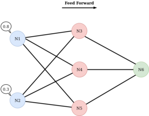
The values are then transmitted to the neurons of the next layer through the connections:
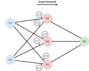
The neurons in the second layer merge the values from the neurons in the previous layer. The resulting merged value can then be modified internally by the neuron:
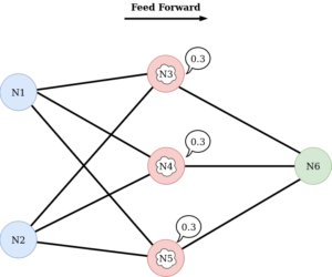
Then, the neurons in the second layer transmit the modified value to the next layer in turn:
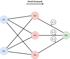
Similarly, the neuron(s) in the final layer (outputs) can internally modify the received value before returning it:
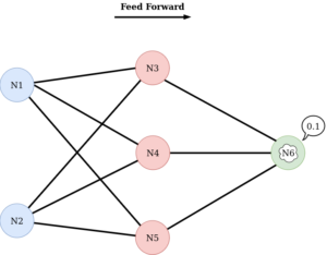
Once the final value is obtained, the feed forward pass is complete.
In reality, the transmission of values is a bit more complex. This is what we will detail next. To properly understand the transmission, we will limit ourselves to 3 neurons.
The transmission of values depends on the “thickness” of the link between the neurons. The thicker the link, the more the value passes through in its entirety, and vice versa. This thickness is called the weight or weight and is different for each link, as seen in the following image:
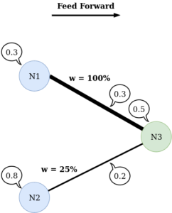
Thus, each neuron does not have the same weight or the same importance within the network.
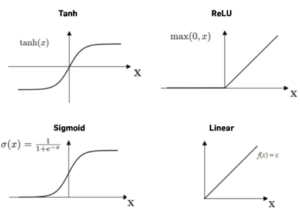
We will now see how the neuron can internally change the value it receives before transmitting it. Specifically, the neuron possesses a function, known as an activation function, which serves to determine whether or not the value should pass to the next neuron. If the result of the function is close to 1, the value will pass; if it is close to 0, the value will not pass.
There are a multitude of activation functions, but the most commonly used are:
– Sigmoid
– Rectified Linear Unit (ReLU)
– Hyperbolic Tangent (tanh)
– Linear
The neuron also has the possibility of adding a bias to the input of the activation function, which allows the neuron to influence the activation:
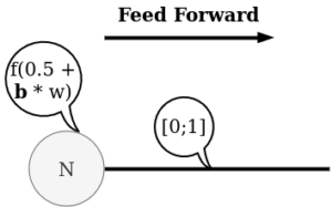
To summarize:
– we have a set of neurons
– we enter the data into the input neurons
– we link the layers of neurons with a certain weight
– we add biases, which are multiplied by their own weight
– we add the values to obtain the new values
– we pass the new values through the activation function
– we repeat the process for the final neuron
We finally obtain the result.
However, since we initialize the biases and weights randomly, there is little chance that the network will be high-performing initially.
We then pass our result into an error function. This function takes our result and the expected value as input. This allows us to determine the accuracy of our network.
We then perform the second step: the back propagation pass. In very simple terms, this step consists of determining how we must modify the weights of our network to minimize our error as much as possible. In practice, we modify one weight at a time, and only slightly, to determine the influence of each weight on our network based on its impact on the error. This step is carried out using the derivatives of all the calculations made during the feed forward phase.
Conclusion
We have discovered what lies behind a neural network, its basic operation, and its various applications. Neural networks offer many possibilities for the field of geomatics through the analysis and interpretation of spatial data. Their ability to learn from raw data makes them a powerful tool for prediction, classification, and even the generation of new geospatial data. However, it is essential to remember that, despite their potential, neural networks are not a miracle solution and can present challenges in practice. In particular, it is important to reiterate that the quality and quantity of data are paramount to obtaining reliable and meaningful results. Finally, it is also essential to note that the effective use of neural networks often requires high computing power and large datasets.
Author: Mathilde POMMIER