Tutorial: Effectively Train My First Neural Network

After learning how to create your first neural network in the article My First Neural Network and studying the theory of model optimization in the article Simple Neural Network Optimization, it’s now time to practice effectively training a neural network! 🚀

To do this, we will revisit the model creation from the article My First Neural Network. We will perform several training sessions to determine the importance of the learning rate in model training. If you have any doubts about the concept of learning rate, the article Simple Neural Network Optimization is there to guide you.

Notebook Preparation

Great! Let’s start by performing all the installations and imports we’ll need for this tutorial. We’ll once again use Jupyter for development.

Create a Python virtual environment (unnecessary if you already created one for the article My First Neural Network):

python3 -m venv test_ia

Activate the Python virtual environment:

cd test_ia
. bin/activate

Install Jupyter and launch it:

pip install jupyter
jupyter notebook

The last command automatically opens Jupyter in your browser. You then just need to create a Notebook by going to “File” → “New” → “Notebook”. Then copy the following code into the Notebook.

Installations & Imports ^*1

^*1: This step was also done in the first tutorial described in the article My First Neural Network.

First, we need to install the following libraries:

• PyTorch, one of the main Python libraries for neural networks. Here we are only installing the CPU version; the base version works with CUDA, Nvidia’s scientific computing library, but it takes up a lot of disk space, so let’s be frugal.
• Pandas, the star Python library for data science, itself based on Numpy (for list management).
• Matplotlib, for creating nice graphs.

!pip3 install torch --index-url https://download.pytorch.org/whl/cpu
!pip install pandas
!pip install matplotlib

Once the installations are complete, we can proceed to import these libraries or specific elements from them.

import torch
import torch.nn.functional as F
import pandas as pd
import matplotlib.pyplot as plt
from random import randint, seed
# Nous n'avons pas eu besoin d'installer random car c'est une bibliothèque standard de Python

Everything is now in place to start the tutorial well!

Creating a Dataset

The first step to training our model is to create a dataset suitable for our problem, on which we can train our model.

This time, we’ll use the example of a skier at the bottom of a mountain climbing up to its summit.

Therefore, we need a dataset that represents the slope of this mountain to train our model.

For this example, we will use a very simple, linear slope with the equation f(x) = 2x. So, this function, a simplified version from the previous article, is what we will use to create our dataset.

data = pd.DataFrame(columns=["x", "y"],
                    data=[(x, x*2) for x in range(10)],
                   )
data["x"] = data["x"].astype(float)
data["y"] = data["y"].astype(float)
# On peut visualiser le jeu de données d'entraînement ci-dessous
plt.figure(figsize=(25, 5))
plt.margins(0)
plt.scatter(data["x"], data["y"], alpha=0.5)
plt.title("Jeu de données d'entraînement")
plt.xlabel("Position x")
plt.ylabel("Altitude y")
plt.grid(True)
plt.show()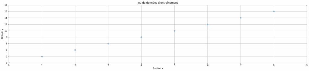

Creating Our Model

Now that our dataset is ready, we can proceed to create our model.

We will create a very simple model because our problem is not very complex. Indeed, the slope of our mountain is linear; consequently, our model only needs one layer of neurons. To create it, we will use PyTorch with a fixed seed to ensure reproducible results.

torch.manual_seed(1337)
seed(1337)
M = torch.randn((1,1))
M.requires_grad = True
print(M)

Training Our Model

With our model and dataset ready, we can now proceed to train the model.

To train our model, we still need to define two variables: epochs and lr.

• epochs represents the number of times the model is trained on a data sample
• lr is the abbreviation for learning rate and represents the rate at which the model’s weights are updated during gradient descent (backward pass or backward propagation)

epochs = 700
lr = 0.1
losses = list()
for epoch in range(epochs):
    # On sélectionne un point de données aléatoire parmi les 10 du dataset
    # Cela permet de varier les données vues à chaque epoch
    ix = randint(0, len(data) - 1)
    x = data.iloc[ix]["x"]
    y = data.iloc[ix]["y"]
    # Forward pass
    y_prevision = M @ torch.tensor([x]).float()
    # Calcul de la loss (perte)
    loss = F.l1_loss(y_prevision, torch.Tensor([y]))
    # Backward pass
    M.grad = None
    loss.backward()
    # Mise à jour du learning rate et de M
    lr = 0.1 # On conserve le même learning rate
    M.data += -lr * M.grad
    # stats : on stocke la loss pour suivre la progression de l'entraînement
    losses.append(loss.item())

Displaying and Interpreting Results

During training, we stored the loss for each epoch; we can now visualize how this loss evolved throughout the model’s training.

plt.figure(figsize=(25, 5))
plt.margins(0)
plt.plot(range(epochs), losses, linestyle='-', color='b', label="Loss")
plt.xlabel("Epochs")
plt.ylabel("Loss")
plt.title("Évolution de la loss au fil des epochs")
plt.legend()
plt.grid(True)
plt.show()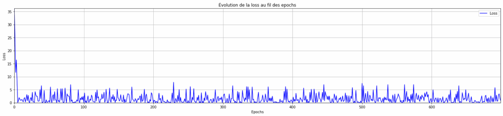

We observe that our model converges very quickly, but still struggles to stabilize (the magnitude of the oscillations remains identical throughout training).

We can also see the impact on data predictions. In other words, are the predictions close to the actual slope? To do this, simply apply our trained model to the initial dataset.

predictions = []
for x in data["x"]: # Pour chaque x du jeu de données original
    y_pred = (M * x).item() # On applique notre modèle entraîné : y = M * x
    predictions.append((x, y_pred))
plt.figure(figsize=(25, 5))
plt.margins(0)
plt.scatter(data["x"], data["y"], alpha=0.5, label="Données réelles")
plt.plot([x[0] for x in predictions], [y[1] for y in predictions], label="Prédictions", color='r')
plt.title("Données réelles vs Prédictions")
plt.xlabel("Position x")
plt.ylabel("Altitude y")
plt.grid(True)
plt.legend()
plt.show()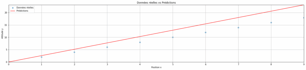

We can see that our model makes predictions quite close to the real data, but they are not entirely accurate. Let’s see if we can improve our training.

Alternative Model Training

To improve our model’s predictions, we can try adjusting the learning rate.

For our first test, we used a high learning rate (0.1), which means that at each iteration, the model’s parameters (weights and biases) are greatly adjusted (which explains the oscillations in the loss).

So, we will now attempt the same training, but with a low learning rate (0.001).

torch.manual_seed(1337)
seed(1337)
M = torch.randn((1,1))
M.requires_grad = True
print(M)
epochs = 700 # On conserve le même nombre d'epochs que pour le modèle précédent
lr = 0.001 # On choisit un learning rate plus faible pour voir son impact sur la convergence du modèle
losses = list()
for epoch in range(epochs):
    # Échantillon aléatoire
    ix = randint(0, len(data) - 1)
    x = data.iloc[ix]["x"]
    y = data.iloc[ix]["y"]
    # Forward pass
    y_prevision = M @ torch.tensor([x]).float()
    # Calcul de la loss
    loss = F.l1_loss(y_prevision, torch.Tensor([y]))
    # Backward pass
    M.grad = None
    loss.backward()
    # Mise à jour
    lr = 0.001 # On conserve le learning rate faible
    M.data += -lr * M.grad
    # stats
    losses.append(loss.item())
# Prédictions finales pour les comparer avec les données réelles plus tard
predictions = []
for x in data["x"]:
    y_pred = (M * x).item()
    predictions.append((x, y_pred))
# Visualisation de la loss en fonction des epochs
plt.figure(figsize=(25, 5))
plt.margins(0)
plt.plot(range(epochs), losses, linestyle='-', color='b', label="Loss")
plt.xlabel("Epochs")
plt.ylabel("Loss")
plt.title("Évolution de la loss au fil des epochs")
plt.legend()
plt.grid(True)
plt.show()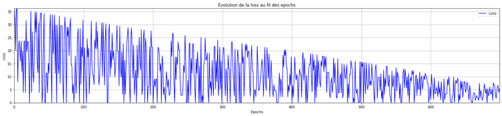

We can observe that with a low learning rate, the model does not converge in 700 epochs (we still have a downward slope and no plateau).

A low learning rate means that at each iteration, the model’s parameters (weights and biases) are modified very little. We try to make small adjustments to them to converge with as few oscillations as possible at the end of training.

Therefore, to converge with a low learning rate, we need a higher number of epochs, simply to allow the model time to converge. Consequently, we will retry the previous training, but this time, with 1000 epochs.

torch.manual_seed(1337)
seed(1337)
M = torch.randn((1,1))
M.requires_grad = True
print(M)
epochs = 1000 # On augmente le nombre d'epochs pour voir si le modèle fini par converger avec un learning rate faible
lr = 0.001 # On conserve le learning rate faible
losses = list()
for epoch in range(epochs):
    # Échantillon aléatoire
    ix = randint(0, len(data) - 1)
    x = data.iloc[ix]["x"]
    y = data.iloc[ix]["y"]
    # Forward pass
    y_prevision = M @ torch.tensor([x]).float()
    # Calcul de la loss
    loss = F.l1_loss(y_prevision, torch.Tensor([y]))
    # Backward pass
    M.grad = None
    loss.backward()
    # Mise à jour
    lr = 0.001
    M.data += -lr * M.grad
    # stats
    losses.append(loss.item())
# Prédictions finales pour les comparer avec les données réelles plus tard
predictions = []
for x in data["x"]:
    y_pred = (M * x).item()
    predictions.append((x, y_pred))
# Visualisation de la loss en fonction des epochs
plt.figure(figsize=(25, 5))
plt.margins(0)
plt.plot(range(epochs), losses, linestyle='-', color='b', label="Loss")
plt.xlabel("Epochs")
plt.ylabel("Loss")
plt.title("Évolution de la loss au fil des epochs")
plt.legend()
plt.grid(True)
plt.show()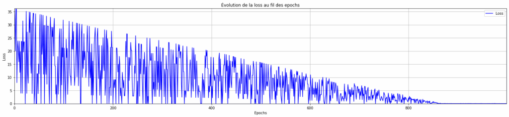

Here, we can see that with a low learning rate (0.001) but a large number of epochs (1000), the model does eventually converge.

But are the model’s predictions more accurate? That’s what we’ll see next.

plt.figure(figsize=(25, 5))
plt.margins(0)
plt.scatter(data["x"], data["y"], alpha=0.5, label="Données réelles")
plt.plot([x[0] for x in predictions], [y[1] for y in predictions], label="Prédictions", color='r')
plt.title("Données réelles vs Prédictions")
plt.xlabel("Position x")
plt.ylabel("Altitude y")
plt.grid(True)
plt.legend()
plt.show()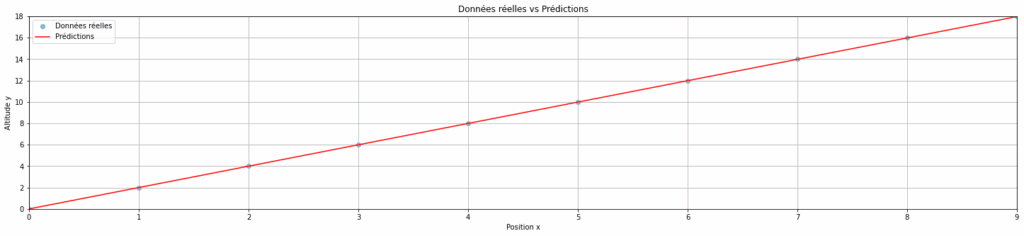

As we can see in the graph above, the model’s predictions are indeed better with a low learning rate! 🎉

Optimal Model Training

As seen previously, training with a high learning rate and a low learning rate both have their advantages and disadvantages.

On one hand, a high learning rate allows the model to converge very quickly, but with large oscillations, which can sometimes mean the loss never stabilizes and thus the model can make poor predictions. On the other hand, a low learning rate ensures a stable loss at the end of training, but with a large number of epochs, leading to longer training and higher computational cost.

To get the best of both worlds, we will try training our model with an adaptive learning rate: high initially to converge quickly, then low to stabilize the loss.

torch.manual_seed(1337)
seed(1337)
M = torch.randn((1,1))
M.requires_grad = True
print(M)
epochs = 150 # On repasse à un nombre d'epochs faible
lr_initial = 0.1 # On commence à un learning rate élevé pour converger rapidement
lr_final = 0.001 # On fini à un learning rate faible pour stabiliser la loss
losses = list()
for epoch in range(epochs):
    # Échantillon aléatoire
    ix = randint(0, len(data) - 1)
    x = data.iloc[ix]["x"]
    y = data.iloc[ix]["y"]
    # Forward pass
    y_prevision = M @ torch.tensor([x]).float()
    # Calcul de la loss
    loss = F.l1_loss(y_prevision, torch.Tensor([y]))
    # Backward pass
    M.grad = None
    loss.backward()
    # Mise à jour
    if epoch < 50:
        lr = lr_initial # Pour les 50 premières epochs, on conserve le learning rate initial (élevé : 0,1)
    else:
        lr = lr_final # Passé la barre des 50 premières epochs, on passe à au learning rate final (faible : 0,001)
    M.data += -lr * M.grad
    # stats
    losses.append(loss.item())
# Visualisation de la loss en fonction des epochs
plt.figure(figsize=(25, 5))
plt.margins(0)
plt.plot(range(epochs), losses, linestyle='-', color='b', label="Loss")
plt.xlabel("Epochs")
plt.ylabel("Loss")
plt.title("Évolution de la loss au fil des epochs")
plt.legend()
plt.grid(True)
plt.show()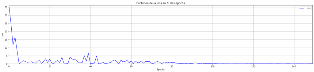

We observe that with an adaptive learning rate, the model converges very well and the loss stabilizes in a very low number of epochs!

So, an adaptive learning rate is a better solution (in terms of efficiency and performance) for training a model. The training cost is lower, and the model makes better predictions.

This adaptation function is actually called a scheduler, and it serves to dynamically adjust a training hyperparameter. In our case, the hyperparameter is the learning rate, so we speak more specifically of an lr scheduler.

For our lr scheduler, we created a very simple function. We start with a high learning rate, then, after 50 epochs, we switch to a low learning rate.

However, we could also improve this function by adapting our learning rate based on the last calculated loss (and not the epoch, which is a somewhat naive variable): as long as the loss decreases, we keep the current learning rate; otherwise, we divide it by two. Feel free to test this version on your own if you’d like!

Conclusion

To conclude, in this tutorial, we explored the concepts of learning rate and scheduler, fundamental aspects of neural network training.

Through different training sessions, we observed that:

✅ The backward pass allows adjusting model parameters by minimizing a loss function.

✅ The choice of learning rate is crucial: too high, the loss is unstable; too low, it becomes too slow.

✅ An adaptive learning rate accelerates convergence initially and stabilizes learning afterward.

✅ There are several ways to adapt the learning rate, and the functions for adapting it are called schedulers.

Feel free to try out this tutorial on your own to master neural network creation and training. For example, you can test different learning rates or lr schedulers for your model’s training! 🚀

---

Author: Mathilde POMMIER, Neogeo